Avenza Announces 2010 MAPublisher Training Schedule

NewsJanuary 4, 2010

– New Class Features MAPublisher Flash Map Creator, Geospatial PDF Export and LabelPro –

Toronto, ON, January 4, 2010 – Avenza Systems Inc., producers of MAPublisher cartographic software for Adobe Illustrator and Geographic Imager spatial tools for Adobe Photoshop, is pleased to announce the 2010 schedule for its comprehensive 2-day MAPublisher training course. This 2-day class offers in-depth MAPublisher training that will enable MAPublisher users to maximize their use of MAPublisher and fully exploit its features and power.

MAPublisher training is offered in hands-on computer labs at locations around North America. Training is also available onsite at customers’ locations and online in which case certain aspects of the course will be tailored especially for the specific organization and workflow.

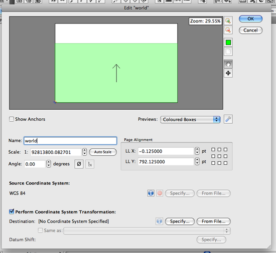
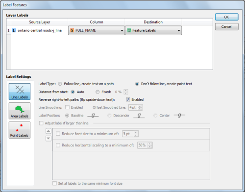
Features of the 2010 round of MAPublisher classes include content on creating interactive data-rich Flash maps, geospatial PDF export and MAPublisher LabelPro advanced text placement.

“I did find the training session very informative and I did learn a fair amount in those two days. I am impressed with the capabilities of MAPublisher and I will definitively recommend MAPublisher and the training session to any of my colleagues working in the map design industry”, said Carlos Serpas of SAIC Polytechnic.

2010 MAPublisher Training Dates & Locations

San Francisco, CA – February 4-5
Washington, DC – March 18-19
Tampa, FL – May 13-14
San Diego, CA – July 15-16
Philadelphia, PA – September 9-10
Denver, CO – November 4-5

For more information and to access the registration form visit the MAPublisher training page.

Course details

The cost is US$1,000 per person. Discounts are available for 3 or more attendees from the same organization.
This is a hands-on course in a computer lab. Computers and required software will be provided.
Attendees will learn how to use the most powerful features of MAPublisher as well as all the new features of MAPublisher 8.
MAPublisher for Illustrator on Windows is the focus of the course. Mac users will also benefit from the content and are encouraged to attend.
Attendees are encouraged to send in and/or bring their own data and time will be devoted to working with specific user-supplied data and workflows.

Who Should Attend

cartographers using GIS data
existing MAPublisher users who want to experience the new features of the latest version of MAPublisher
existing MAPublisher users who want to get the most out of their MAPublisher license
GIS professionals who want to produce better quality maps
anyone making maps that wants to leverage the benefits of this powerful software

More about MAPublisher

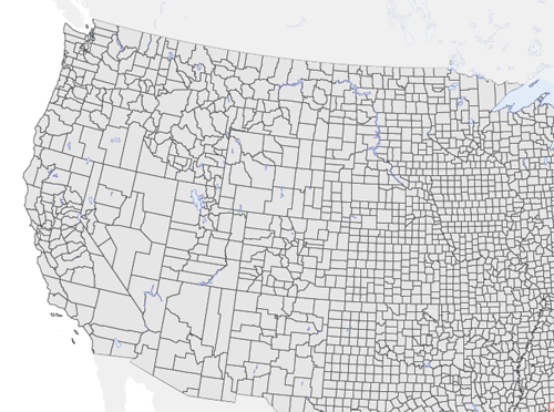
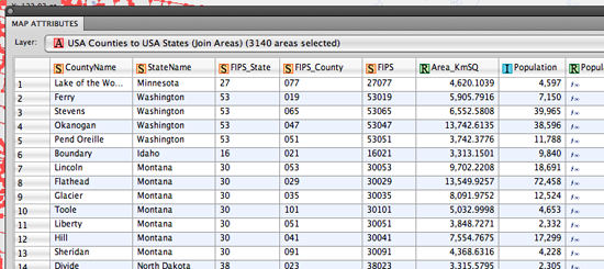
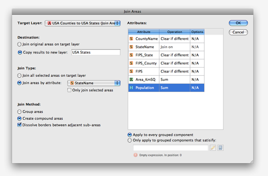
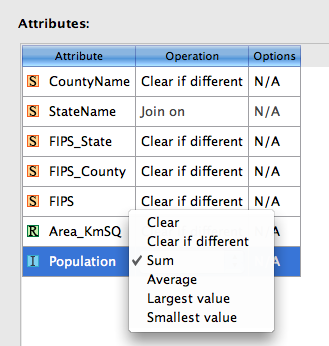
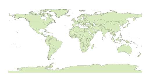
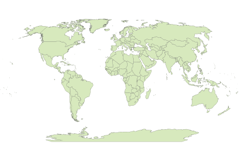
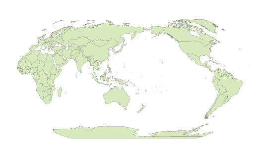
MAPublisher for Illustrator is powerful map production software for creating cartographic-quality maps from GIS data. Developed as a suite of plug-ins for Adobe Illustrator and Macromedia FreeHand, MAPublisher leverages the superior graphics capabilities of these graphics design applications. Full details are available at www.avenza.com/mapublisher

More about Avenza Systems Inc.

Avenza Systems Inc. is an award-winning, privately held corporation that provides cartographers and GIS professionals with powerful software tools for making better maps. In addition to software offerings for Mac and Windows users, Avenza offers value-added data sets, product training and consulting services. Visit www.avenza.com for more details.

For further information:
Avenza Systems ● 416-487-5116 ● info@avenza.com ● www.avenza.com

New Join Areas feature in MAPublisher 8.4

BlogDecember 28, 2010

The upcoming release of MAPublisher 8.4 introduces many new features. One of the new features is called Join Areas. We have received a lot of requests from our customers to create area objects by merging common attribute values. This geoprocessing function is generally known as “dissolve”.

The picture below shows polygon objects from a USA Counties layer. The goal is to create a layer with state boundaries and summing the population count by joining the objects of the counties layer.

In the MAP Attributes panel of the USA Counties layer, every object of the counties layer contains attribute information including county name, state name, FIPS codes, area in km², population and so on. We’ll be using the StateName attribute value to combine all the county polygons into one polygon per state.

This is the new Join Area dialog box. On the left side, we’ll specify 1) target layer, 2) destination (output) layer, 3) join type and 4) join method. We are trying to create state boundaries from the counties target layer so we’ll select a join type based on the StateName attribute and output it to a new layer called USA States. The join will create compound paths and since our goal is to create state polygons, we’ll dissolve borders between adjacent sub-areas.

On the right side of the dialog box are attribute value operations available for each column. These operations determine what kind of the values will result for every attribute and the operations available are different for each data type (String, Real, Integer). The screenshot below shows the attribute value operation set to Sum for Population attribute (Integer data type). When the Join Area is complete, each state polygon will have the sum of the population of all the counties that belong to it.

After running the Join Areas function, county polygons are dissolved into state boundaries.

The population values show the total sum from all the counties for every state.

This is just one example of how Join Areas can be used. It was initially a feature request and with some discussion and planning, it became real. If you have any feature requests for MAPublisher, Geographic Imager or PDF Maps, please feel free to drop us a line at support@avenza.com. We’re happy to hear from all of you!

New Transformation Method for World Maps in Geographic Imager 3.2

BlogNovember 29, 2010

When transforming a world image, there may be artifacts created by the Geographic Imager transformation engine. Below are the results of a WGS84 world image transformed into a Stereographic projection.

When we zoom into the problematic area, you can see up close how some artifacts affect the image after the transformation was performed.

To solve this issue, we are introducing a new projection method called Maximum: World Projection in Geographic Imager 3.2.

We are going to use the same world image used with the previous example and transform it into the stereographic projection. Take a close look at the Advanced Options.

Under the Performance/quality section, select Maximum / World Projections from the Precision drop-down list and click OK.

Below is the result of the transformation with the new method available in Geographic Imager 3.2.

Let’s take a close look at the same area where the problem happened with the previous version of Geographic Imager. Now the transformed image does not contain any artifacts.

This option is available since Geographic Imager 3.2. The official version of Geographic Imager 3.2 is available now.

Making dashed lines intersect at every intersection in MAPublisher

BlogDecember 7, 2010

One of the great advantages of using Adobe Illustrator for a mapping project is that you can make great line styles easily. For example, to make a double line stroke and one of them is dashed:

Double strokes are a line graphic style where two different line strokes overlap each other. For example, the image shows that there is a stroke with a brown color and its stroke size is 3 pts. On top of this brown line, there is a 1 pt white dash line:

You might have an experience where you duplicated one line layer and assigned a different style for lines in each of those layers. However, this has some disadvantages. The file size will increase because all the line segments as well as the attribute information attached to every line object is duplicated. Also, when you apply the double stroke line to road layer, the white dash line does not intersect nicely at every intersection of the map:

With Adobe Illustrator CS5, these problems are solved.

0) Create a graphic style like the one shown above.

1) Open the Pathfinder panel (Window > Pathfinder).

2) Select all the line objects in the line layer.
Click the outline tool .

This function in the Pathfinder tool breaks lines at every intersection.

All the selected objects which were selected at Step 2 will be broken into segments at every intersection and they will be grouped as one object in the layer.

3) Having the grouped objects selected, apply the graphic style with the double stoke.

4) The white dashed line is intersected at every intersection nicely.

Quick tip

When creating double stroke, make sure to select the option “Align dashes to corners & path ends, adjusting length to fit” available next to the dash line option.

Note

Since this operation involves a pathfinder functions, the attribute information will not be matintained after the “outline” function is applied to those selected line works. Our development team is looking for a possible solution to keep the attribute information for the future version of MAPublisher.

Changing the Point Angle using Expressions and Attribute Values in MAPublisher

BlogNovember 29, 2010

Here we have placed point symbols for a MAP Point layer. However, we want to change the point angle using the Attribute values.

Below is the attribute table for the point data shown above. The field directionAngle is the field containing the symbol rotation value. With MAPublisher, it’s possible to assign this value to every symbol in this layer.

Open the Edit Schema dialog box from the MAP Attribute panel. Find the field called #Rotation from the attribute field list. This #Rotation field is hidden/invisible by default. Click the Visible option to enable it and click OK.

In the MAP Attributes panel, you can see that the #Rotation field shown. The values in this field is 0.00 degree for every point in the layer. We’ll assign the angle value from the directionAngle field to the #Rotation value .

Open the Apply Expression dialog box from the MAP Attributes panel. Enter the column name directionAngle for the Expression and ensure that the value will be applied to the field #Rotation.

Every value from the directionAngle field is now inherited by the #Rotation field.

As a result, the rotation angle is now applied to every point.

The origin of the rotation is at each point’s registration point. With Adobe Illustrator CS4 and earlier, the registration point is set at the centre of the point symbol. With Adobe Illustrator CS5, the registration point can be flexibly placed. This will be discussed with some examples in a later topic. Stay tuned!

Creating a Custom Coordinate System from a Predefined Coordinate System

BlogOctober 13, 2010

When transforming a world map in a geodetic system (such as WGS84) to a predefined projection (such as Robinson) using MAPublisher, the central meridian of the predefined projection should be set to 0 degree longitude as shown below.

Image 1: world map in WGS84

Image 2: world map in a predefined Robinson Projection

However, you might want to have a map with a different region centred on your map. For example, Image 3 below shows a world map with a part of Asia centred. In this case, the central meridian was set to 160 degrees East.

Image 3: world map in a custom Robinson Projection with a central meridian value set to 160 degree East

Today we’ll introduce how to create a custom coordinate system by modifying a predefined coordinate system. We’ll use an example using a GIS dataset world.mif available in the MAPublisher Tutorial folder. We are going to transform a world map to a custom central meridian value with the Robinson projection.

Step 0 : import the “world.mif” file from MAPublisher tutorial folder.

Step 1 : Open the MAP View Editor window from the MAP Views panel.

In the MAP View Editor window, you can see that the scale of the map, position of the map extent with respect to the current document extent, and most importantly the current coordinate system assigned to the MAP View.

We are going to transform the MAP View from WGS84 to the Robinson projection with a custom central meridian value. Check the “Perform cordinate System Transformation option.

Click the Specify button under the “Perform Coordinate System Transformation” section. It will open the “Specify Destination Coordinate System” dialog box.

Step 2: Creating a custom coordinate system with the Robinson projection

We are going to create a custom coordinate system based on the Robinson projection by modifying the existing Robinson projection. Find the existing Robinson projection from the list.

On the left side, navigate to Coordinate system > Projected > World. Highlight the folder “World”. You will see the list of the predefined coordinate systems available on the right side of the window. Find the “Robinson” and highlight it.

Once the predefined Robinson projection is highlighted, click the Copy button at the bottom. It will duplicate the existing coordinate system and will open the “Projected Coordinate System Editor” dialog box for the duplicated coordinate system.

In the Projected Coordinate System Editor dialog box, there are two tabs: Identification and Definition. In the Identification tab, enter a new name for this customer coordinate system. This name will be used when you are searching the object.

Click the Definition tab. Change the value of central_meridian from 0 (default) to 160. Click OK to apply this new setting. You have just made a custom coordinate system based on the existing Robinson projection.

Step 3: Complete the Transformation

Under the “Perform Coordinate System Transformation”, the new custom coordinate system just created is indicated. Now you are ready to transform your map.

Now the world map is successfully transformed into the custom coordinate system (Robinson with the central meridian set to 160 degree East).

You might want to take a look at this other blog about the new transformation engine implemented in MAPublisher 8.3.

Transforming an image into a custom coordinate system with Geographic Imager

You can use the same approach to transform your image into a custom coordinate system.

First, we open a world image that has a WGS84 coordinate system.

Click the Transform button in the Geographic Imager main panel. It will open the Transform dialog box.

Click the Specify button. Now repeat Step 2 illustrated above to create a custom coordinate system. Once you select the custom coordinate system in the “Specify Coordinate System” dialog box, it will be indicated in the Transformation dialog box (in the example below, a custom coordinate system “Robinson cm @ 160 degree East” is selected as a destination coordinate system).

As soon as you click the Transform button, the transformation process will start. Once the transformation process is completed, the Geographic Imager main panel will indicate the new custom coordinate system name.

Working with Custom Highway Shield Symbols and Label Features

BlogAugust 19, 2010

MAPublisher offers a variety of labelling options, ranging from the MAP Tagger tool used for hand labelling single pieces of art, the Label Features tool for automatic attribute labelling, and MAPublisher LabelPro™, a separately licensed advanced labelling engine.

MAPublisher LabelPro ships with nearly 100 highway shields from across North America into which attribute labels can be easily placed. Although LabelPro does not support adding custom symbols to its existing symbols library, the following instructions outline a manual method for adding a custom highway shield to your map, along with placing text on to this shield.

First we must setup our custom shield. This can be drawn in Adobe Illustrator, or produced from a pre-existing image brought into Illustrator using the File > Place menu option. For this exercise I have taken a highway shield I found online from York Region Ontario, and using Adobe Photoshop removed the highway number from the shield.

Once the shield is drawn and sized appropriately and placed in Illustrator, simply use the Selection Tool to drag the symbol into the Adobe Illustrator Symbols panel. Be sure to name the symbol, as you will need to access the symbol from a list later on; I named mine “York_Shield”

Our next step is to produce our feature labels. Using the Label Features tool, choose to label with the “Don’t follow line, create point text” option selected. Once the labels are placed on the map, use the Adobe Layers panel to select the labels and use the Paragraph panel or the Control Toolbar to centre justify the labels. This step is important for easily lining up our shields with the labels.

We now need to create a point layer with a point corresponding to each label. This is easily done by using the MAP Attribute panel option menu to “Export Attributes..” of our newly created Feature Labels MAP Text Layer. Be sure to choose export all attributes under Options: Scope, and to check “Include column names on first line” as we will be using the hidden MAPX and MAPY attribute columns when importing this data back into the map as point data.

Next, use the MAPublisher Simple Import tool to add the newly created .csv file of referenced attribute information. When prompted by the Settings dialog, choose the MAPX column as the column containng X coordinates, and MAPY for Y coordinates. Once the data is imported, if it has not been added to the MAP View containing your line and text layers, add it, and specify the coordinate system if necessary.

With the imported point data selected, open the MAP Attribute panel and right click a column heading to access the Show/Hide Columns > Show All option. double click the #Style column and change the style to your shield symbol. Use the Apply Expression tool in the option menu to apply the symbol to every item at once.

Alternately, a MAP Stylesheet can be built to apply the symbol only to art with a specific range of attributes. In the Adobe layers panel move your label layer above your symbol layer.

If text and symbol do not line up as desired, the symbol geometry will need to be altered. If you are using CS5, doubble click the shield in the symbol panel to enter isolation mode, here you can drag the symbol to respecify the anchor point so that your symbol lines up as you would like it. If you are using CS3 or CS4, you will need to add some invisible art (no stroke/no fill) just below or above the symbol to adjust its extents, and where exactly the symbol’s centre point is located. As well, symbol and text rotation can be edited globally by changing the #Rotation attribute in the MAP Attributes panel.

Geographic Imager 3.2: Introduction to Terrain Shader, Part 3 – Applying Terrain Shader to multiple DEM files

BlogAugust 17, 2010

If your workflow involves Terrain Shader, specifying a DEM schema is an important step, especially when dealing with mulitple DEM files.

When importing a single DEM file, Geographic Imager converts elevation values to gray scale values. For example, if the elevation range in your DEM file is between 0 and 2500 meters and the “Auto-stretched” option is selected, this range will be converted to the Adobe Photoshop gray scale range between black and white. As shown below, the black color is assigned to the lowest elevation value (0 meter) while the white color is assigned to the highest elevation value (2500 meters). For elevation values between 0 and 2500, Geographic Imager calculates and converts them into gray scale.

In this example, we’ll use six DEM files of one geographic region. Many datasets are distributed as tiled DEM files. Each of them is next to each other and the goal is to create a colorized DEM image from those six files.

When dealing with multiple DEM files, you will need to consider the elevation range of the each DEM file. In other words, the elevation range in each DEM file will be slightly different.

Option 1: Using the “Auto-Stretched” option for multiple DEM files

When importing multiple DEM images and using the “Auto-stretched” option, click “Apply to All”…

Every one of the DEM images will be converted to the gray scale between black and white.

As a result, you can get the maximum contrast in each image. However, you will not be able to mosaic or apply Terrain Shader to those six images because each DEM has slight differences in elevation and an all encompassing schema like the”Auto-stretched” option will not work.

Option 2: Creating a DEM schema by specifying a range

In order to apply Terrain Shader to multiple DEM files, you will need to assign one DEM schema to each DEM image you would like to share the same schema.

Step 1: Identify the elevation range amongst multiple DEM files

Explore the DEM files and find out what the elevation range is for each one. Then note which are the lowest and highest values among all DEMs. For this example, the lowest elevation is 0 m and the highest is 3,231 meters.

Step 2: Create a new DEM schema for your dataset

Choose File > Open and select multiple DEM files. Once the Import DEM file dialog box is open, click the Add button to open the “Edit DEM Schema” dialog box.

Create a new Schema name (e.g. “my study area”). Simply enter the lowest and highest elevation value found in Step 1.

Step 3: Apply the DEM schema to your datasets

When you’ve created a new DEM schema, it will be available in the “Select Schema” drop-down list. Choose the new schema and click “Apply to All”. This selected schema will be applied to all the DEM files being imported.

After the import process is completed, the images are ready for Terrain Shader.

When one of the imported DEM file is the active document, click the “DEM” tab in the Geographic Imager panel. It shows the DEM schema name, the DEM value range, and the actual elevation value available in the currently active document. Click the “Calculate” button if you do not see the statistics (actual elevation value range of the active document).

Step 4: Apply Terrain Shader to your DEM files

Since each DEM has a schema, a mosaic can be perfomed and then Terrain Shader can be applied to the mosaicked iamge.

Geographic Imager 3.2: Introduction to Terrain Shader, Part 1

BlogAugust 11, 2010

The upcoming release of Geographic Imager 3.2 introduces a new feature called Terrain Shader, used to apply color gradients and shaded relief to imported DEM images. Color gradients can be exported so that you can use them for other images or share them with other people.

You might want to take a look at our brief video about the Geographic Imager Terrain Shader on our Avenza YouTube channel.

In this blog, I’ll show you a quick workflow with Terrain Shader using one of the files from the Geographic Imager tutorial folder.

1) Open the DEM file called Yukon Water.dem from the Geographic Imager Tutorial Folder in Adobe Photoshop. Geographic Imager will automatically detect the file type so that you will see the “Import DEM File” dialog box(below).

When your workflow involves Terrain Shader, it is important to select an appropriate schema in the Import DEM file dialog box. For now, we’ll use the option “Auto-stretched”. We’ll return to this dialog box when we talk about an advanced use of Terrain Shader feature in another blog.

After the DEM file is successfully imported, you will see the geospatial information, the DEM schema and the value range information in the Geographic Imager panel. The panel has been redesigned and improved for version 3.2 (We think it works really well!)

2) Click the Terrain Shader button.

In the Terrain Shader dialog box, on the left side, you can see the elevation range of the DEM file. There is a large preview image at the centre of the dialog box.

3) Click the check box beside “Apply Color Map” to apply a color gradient to the DEM image.

You can select one gradient from the preset gradients from the dropdown menu. Or you can edit the color gradient form the existing one. Click the pencil icon next to the preset dropdown menu. In the Edit Color Map dialog box, you can modify the gradient scheme. You can change colors, add ramps, adjust the ramp position, ….etc.

4) Click OK to apply the modication.

5) Another great function with the Terrain Shader is to apply the shaded relief effect at the same time. Click the check box beside “Applly Shaded Relief”.

You can adjust the angle of the source light and the intensity of the contrast. You can see how the settings affect the DEM image in the preview.

6) The DEM is stylized with a color gradient and a shaded relief effect.

Stay tuned for Introduction to Terrain Shader, Part 2

Geographic Imager 3.2: Introduction to Terrain Shader, Part 2 – Creating shaded relief

BlogAugust 10, 2010

In a previous blog, we showed you how to create a shaded relief image from an imported DEM file by using either our JavaScript to automate all the processes or through a manual method.

With Geographic Imager 3.2, you can produce a shaded relief image using the new feature Terrain Shader quickly and easily with just a few clicks.

We will use the Rocky Mountain.dem file available in the Geographic Imager tutorial folder.

1) Open the Rocky Mountain.dem file in Adobe Photoshop. As mentioned in the previous blog, selecting an appropriate DEM schema is an important step before using the Terrain Shader. For this image, we will choose the “Auto-stretched” option, which will give you an optimum result in Terrain Shader.

2) Click the Terrain Shader button on Geographic Imager main panel.

3) In the Terrain Shader dialog box, uncheck the “Apply Color Map” option and check the “Apply Shaded Relief” option.

4) In the Apply Shaded Relief settings, adjust the light source angle and intensity.

As you adjust the settings, use the preview image to get a sense of what your image will look like.

Now that a shaded relief image is created, lets tweak it a little and make some adjustments.

The shaded relief image looks dark. It is because the blending mode of the shaded relief layer, #GI Shaded Relief Layer, is set to “Overlay” (the drop-down menu in the Layers panel).

5) Highlight #GI Shaded Relief Layer and Change the blending mode to “Normal”.

Alternatively, simply turned off the visibility of the original DEM layer “Rocky Mountain.dem” in the Layers panel.

You will get the same effect. The shaded relief now shows the crisp shading effect.

6) If you want to change the brightness and contrast of the produced shaded relief image, you can simply add an adjustment layer in the Layers panel.

Simply adjust the brightness and contrast values in the Adjustments panel.

Now, the shaded relief image is ready for your map!

As always, when you use Geographic Imager, all the georeference information is maintained while you work with Adobe Photoshop and Geographic Imager functions. This is a great advantage when dealing with geospatial datasets.

One quick note: If you want to use a shaded relief image with MAPublisher in Adobe Illustrator, you may save the shaded relief image with spatial reference information. Before saving the image, go to Image > Mode > 8 Bits/Channels. It will convert the image from 16 bits to 8 bits, which is necessary when working with images in Adobe Illustrator.

To place the image in Adobe Illustrator, use the MAPublisher “Register Image” function to align the image with your vector work.

Using these steps will add a nice texture to your map.

Avenza maps makes it easy to interact with offline
maps on your iOS, Android and Windows devices.

Get the app. Get the map.

Yearly Archives: 2010

Avenza Announces 2010 MAPublisher Training Schedule

2010 MAPublisher Training Dates & Locations

Course details

Who Should Attend

New Join Areas feature in MAPublisher 8.4

New Transformation Method for World Maps in Geographic Imager 3.2

Making dashed lines intersect at every intersection in MAPublisher

Quick tip

Note

Changing the Point Angle using Expressions and Attribute Values in MAPublisher

Creating a Custom Coordinate System from a Predefined Coordinate System

Transforming an image into a custom coordinate system with Geographic Imager

Working with Custom Highway Shield Symbols and Label Features

Geographic Imager 3.2: Introduction to Terrain Shader, Part 3 – Applying Terrain Shader to multiple DEM files

Option 1: Using the “Auto-Stretched” option for multiple DEM files

Option 2: Creating a DEM schema by specifying a range

Geographic Imager 3.2: Introduction to Terrain Shader, Part 1

Geographic Imager 3.2: Introduction to Terrain Shader, Part 2 – Creating shaded relief

News Archive

Avenza maps makes it easy to interact with offlinemaps on your iOS, Android and Windows devices.

Get the app. Get the map.

2010 MAPublisher Training Dates & Locations

Course details

Who Should Attend

Quick tip

Note

Transforming an image into a custom coordinate system with Geographic Imager

Option 1: Using the “Auto-Stretched” option for multiple DEM files

Option 2: Creating a DEM schema by specifying a range

News Archive

Avenza maps makes it easy to interact with offline
maps on your iOS, Android and Windows devices.