Styling a MAPublisher Scale Bar

BlogJuly 30, 2010

After generating a scale bar, it is placed in a MAP Legend layer. You can accept the default look of it, but majority of users will want to customize and style it to match their map.

Now I’ve just generated a simple scale bar. If you expand the Legend layer, you can see the object “MAPublisher Scalebar” is placed within it. This is a special object generated by MAPublisher and there is currently a dynamic link between the MAP View information (i.e. spatial information) and the scale bar object.

In order to make a custom scale bar, you will have to break the dynamic link between MAPublisher and the scale bar object. In your own workflow, it’s important that you setup the scale before breaking the link because it will not rescale dynamically after the link is broken. Break the link by expanding the generated object.

From the main menu, choose Object > Expand.

In the Expand dialog box, click the “Object” check box, then click OK.

The result: the object <MAPublisher Scalebar> is replaced by an object called <Group> in the Layers panel. The connection between the scale bar object and MAPublisher is removed. The art in the scale bar object simply became grouped objects.

At this point, select objects in the group and change its colors and lines by using the direct selection tool . The direct selection tool allows you to select individual object even if select objects is a part of a <Group> object.

If you are more comfortable with the selection tool , you will want to read the suggestion below. It works, too.

Take a look at the Layers panel again more closely. The screen capture of the Legend layer above shows that there is a <Group> object under the “Legend” layer. When the object tree under the “Legend” layer is expanded, you can see another <Group> object nested within a <Group> object. (a <Group> object containing a <Group> object). Since all the objects are still grouped, you can simply “ungroup” the art.

Select the <Group> object (i.e. the scale bar object for this example), then from the main menu, choose Object > Ungroup.

When you ungroup the object once, you now see only one <Group>. This <Group> object contains all the text, lines, and area objects composing a scale bar object.

Now, ungroup the object once more. Finally you do not see the object <Group> anymore under the “Legend” layer. It indicates that every object in the layer can now be selected individually using the direct selection tool.

Select the objects to edit and style them using Adobe Illustrator tools!

Geographic Imager: Create shaded relief from a DEM

BlogJuly 26, 2010

With Geographic Imager 3.x, you can import DEM files to Adobe Photoshop and can create shaded relief images.

There are two methods to achieve this:

Method 1: Run the pre-made JavaScript and apply it to all images

After opening your DEM image, choose File > Scripts > Browse… and select Shaded Relief.jsx from the SampleScripts folder inside the Geographic Imager Tutorial folder. It will generate the shaded relief image for the opened DEM image based on the settings in the JavaScript file.

Method 2: Create shaded relief images manually

We’ll use the DEM file Rocky Mountains.dem available in the Geographic Imager Tutorial folder for this demonstration.

1) Open the Rocky Mountains.dem image from the Geographic Imager tutorial folder. Geographic Imager automatically detects it as a DEM file and provides the option to select the DEM image import method. For this demonstration, choose Auto-Stretched from the Select Schema drop-down list.

The imported DEM is opened in black and white. Take a look at the header of the image (or tab of the image file). Notice that it displays “Gray/16”. This indicates that the image is in the 16 Bits/Channel Grayscale mode.

2) Now, change the image mode from 16 Bits/Channel Grayscale to 8 Bits/Channel RGB. From the top menu bar, choose Image > Mode and then 8 Bits/Channel. Once again, go to Image > Mode, this time choose RGB Color.

Once completed, take a look at the image header again (or file tab). Now “RGB/8” is indicated in the header, meaning that the image is now in the 8 Bits/Channel RGB color mode.

3) Select the entire canvas (use the Rectangular Marquee Tool) and copy the selected area to the clipboard (Edit > Copy).

4) Open the Channels panel (Window > Channels) and add one Alpha channel by clicking the Create new channel button at the bottom of the panel or go to the panel option menu and choose New Channel. Leave the channel name as “Alpha 1”.

5) Select the “Alpha 1” in the Channels panel and fill it in white using the Paint Bucket Tool.

6) In step 3 we copied the selected area (the entire canvas) to the clipboard, now we’re going to paste it to the new channel. Select “Alpha 1” in the Channels panel, and paste it (Edit > Paste). You can see that the same image is displayed for all the channels when the copied area is successfully pasted. Make the Alpha 1 channel invisible and make sure the RGB channels are visible.

7) Deselect the area (Select > Deselect from the top menu bar).

8) In the Layers panel (Window > Layers), create a new layer named Bump map. Change the Blending mode to Overlay.

9) Using the Paint Bucket Tool again, fill the new “Bump map” layer with white.

10) From the menu bar, choose Filter > Render > Lighting Effects…

11) Adjust the settings in the Lighting Effects dialog window.

12) The shaded relief image is completed! You can use this image to overlay with other georeferenced images with Geographic Imager or with vector datasets with MAPublisher.

Buffer Art in MAPublisher

BlogJune 25, 2010

Up to MAPublisher 8.2, the MAPublisher Buffer Lines function was limited to only Line features. For MAPubisher 8.3, a revised buffer function called Buffer Art can be performed on both Line and Point layers. Buffer Art allows you to enter one fixed value to either all or the selected art in one layer or the values from an attribute column in one map layer.

Example 1: Applying a static value for the buffer width

Below is the new Buffer Art dialog box. I have one MAP Point layer with a location of a strong earthquake recorded in India n May 31, 2010.

I specified a value of 2100 Kilometer as the distance to buffer from the epicentre (the origin of the earthquake). The buffered art will be placed in the existing destination layer Buffer Area – 300 km interval.

For the buffered area, a pre-designed graphic style will be applied.

Lastly, I enabled the Add concentric circles every: option. This option will generate evenly spaced rings around the points within the buffered area. I am selecting 300 Kilometer for each concentric circle distance. It will generate seven concentric circles within the 2100 km buffer. As a result, you can see that a concentric ring is drawn every 300 km from the epicentre.

Example 2: Applying values from an Attribute Column for the buffer width (Creating Graduated Symbols for every point)

I will use another point layer this time. I have one MAP Point layer with the point information of earthquake epicenters. The size of the buffer width in the page unit (pixel) was calculated based on the size of the magnitude for every point in the layer. Those values under the BufferCircle column will be used for the buffer width.

Now, the Buffer Art feature will be performed with those calculated values for the buffer width.

The Attribute Value option is chosen and the BufferCircle field for the Buffer Width.

As a result, every buffered area (circle) has a different size. Also, the graphic style selected for the buffer art had some level of transparency applied. You can see the darker color when the buffered art overlaps each other. In other words, the region where the dark orange is observed experienced earthquakes more than once.

Buffer Art can be applied to many situations such as around parcel lots, around road or highway lines or even creating them to find intersection proximity between map features. Experiment with your own to find out what is most useful for your own data.

Create a New MAP View For Adobe Photoshop Paths in MAPublisher 8.3

BlogJune 10, 2010

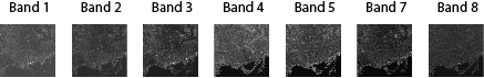
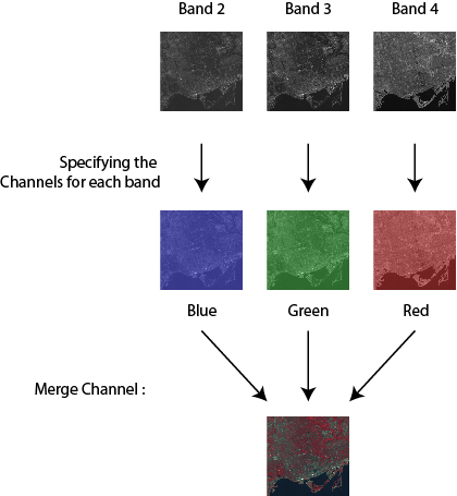
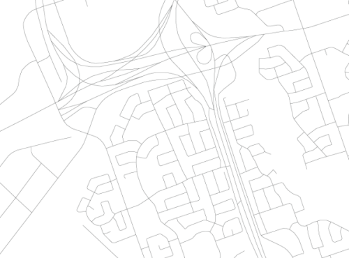
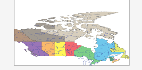
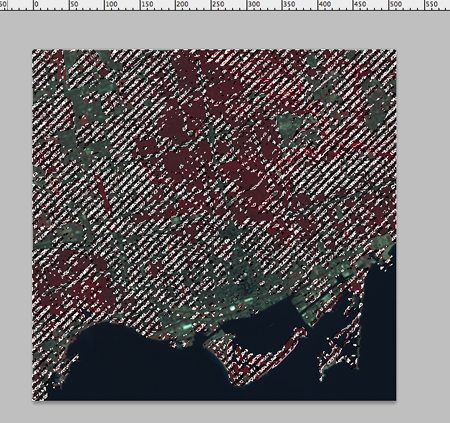
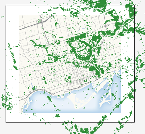
In our previous blog, we introduced you to a quick technique for remote sensing imagery: to depict a type of land types (green area) from a Landsat image. Below is the false composite image created in the previous blog. Basically, the red area indicates a lot of green vegetation (i.e. trees, shrubs, etc).

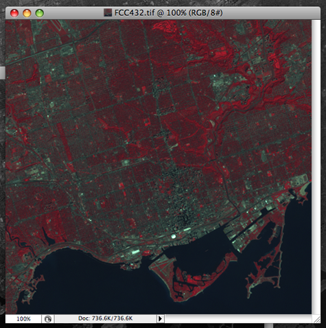
Now, you may be wondering how those red areas can be extracted from Adobe Photoshop and Geographic Imager and brought into Adobe Illustrator and MAPublisher?

An overview of the steps involved in this technique:

In Adobe Photoshop & Geographic Imager:

Select the red areas with Adobe Photoshop tools.
Save the selected pixel areas as “work path”.
Export the saved work path as an Adobe Illustrator file.
Export the georeference information from Geographic Imager option menu.

In Adobe Illustrator & MAPublisher:

Import the exported Adobe Illustrator file with the work path.
Assign the georeference information to the imported work path objects.
If you have already made a map with vector dataset, open the AI file.
Import MAP Objects from the AI file with the workpath to another AI file with a map.
Drag and Drop transformation to align the workpath objects geospatially.

Below are the detailed step-by-step intructions.

In Adobe Photoshop and Geographic Imager:

1. Select the red areas

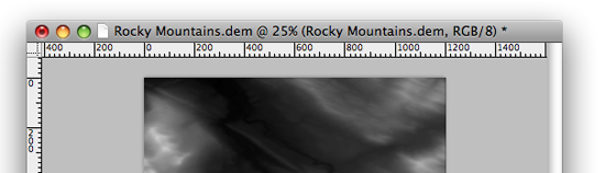
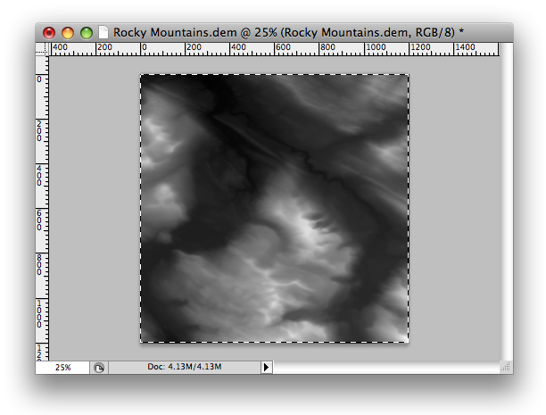
Open the false color composite image in Adobe Photoshop. Now, all the red areas must be selected using any of the following Adobe Photoshop tools.

For example, you can select the red areas using the Magic Wand Tool. You may want to adjust the tolerance values as you begin to select the areas so that only the approriate areas are selected. If you disable the “Contiguous” option from the settings tool bar, it selects all the areas with the same color as the one you collected.

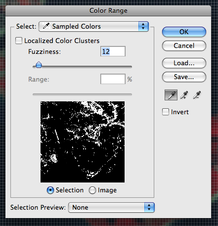
If you want to more precisely select red areas with a preview window, use the Color Range Tool (Select > Color Range). With this tool, sample the color of interest first. In this example, you might want to pick only the areas with the bright red color or you might want to be within a specifc range of red. Using this, you will have more control on which areas are selected.

Of course, there are other techniques you can use to collect the pixels with a specific color. The two suggested above are used quite commonly in our workflows.

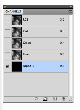
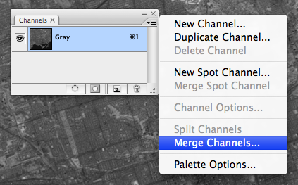
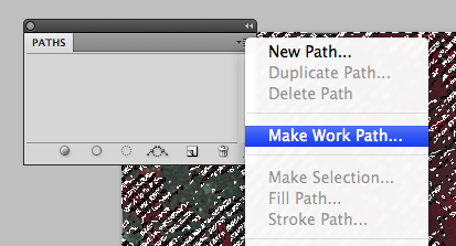
2. Save the selected pixel areas as “work path”

After all the red areas are selected, save the selected area as “work path”. This option is available in the Paths panel options menu.

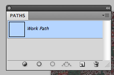
The selection is now saved as a “work path” in the Paths panel.

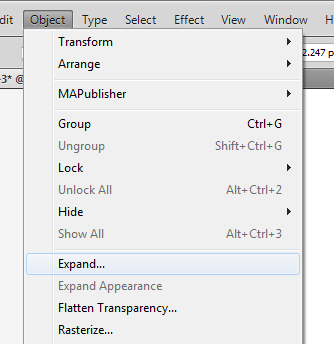
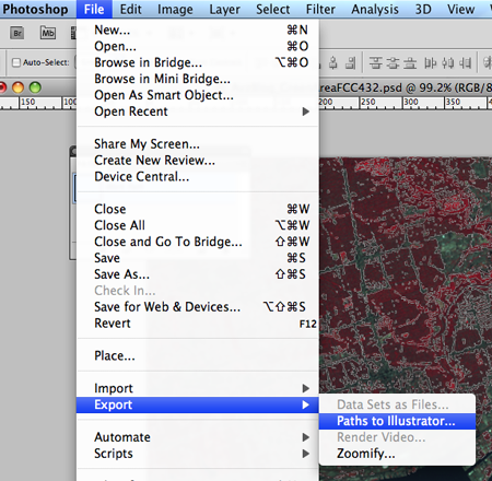
3. Export the saved work path as an Illustrator file

Once the work path is saved in the Paths panel, export it as an Illustrator file (File > Export > Paths to Illustrator).

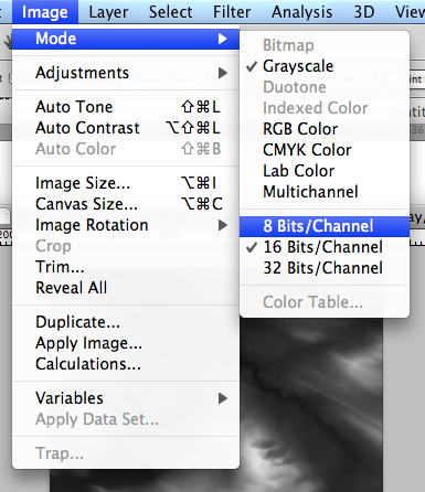
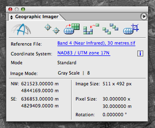
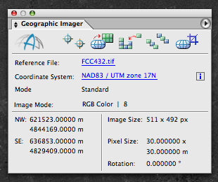
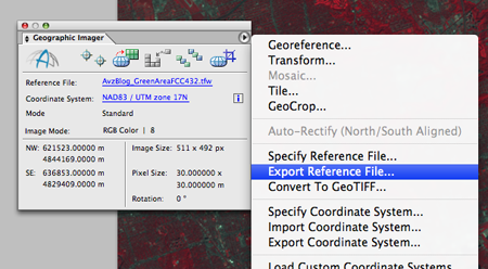
4. Export the georeference information from Geographic Imager option menu

As you saw in the Geographic Imager panel for the false color composite file in the previous blog, this image was georeferenced. Furthermore, we need to export the georeference information that will coincide with the Adobe Illustrator file we just exported.. You can export this georeference information as a MapInfo TAB file or Blue Marble Reference RSF file from the Geographic Imager panel options menu.

In Adobe Illustrator & MAPublisher

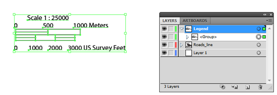
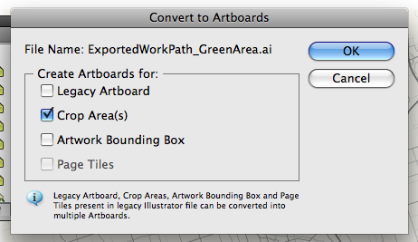
5. Import the exported Illustrator file with the work path

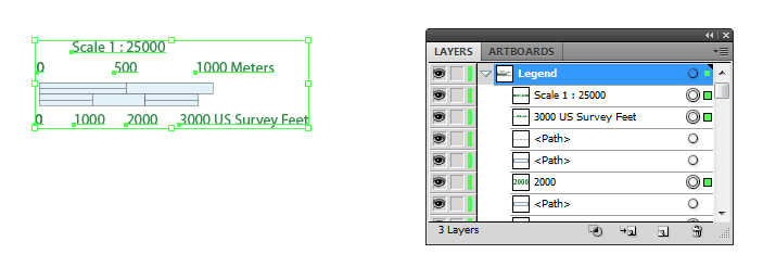
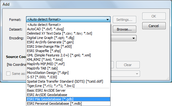
In Adobe Illustrator, open the Adobe Illustrator file exported from Adobe Photoshop (Step 3). Upon opening, a prompt appears to convert the exported file to Artboards. Select the second option “Crop Area(s)”.

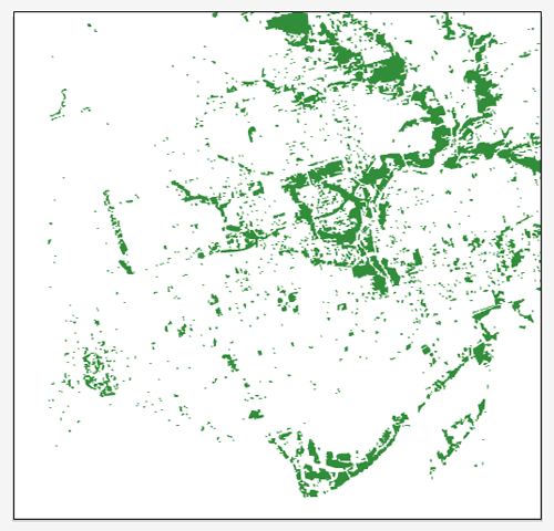
When the artboard is opened, it seems like there is nothing on the artboard. It is simply because there is no color assigned to the fill and stroke. I put a green color for the work path objects.

6. Assign the georeference information to the imported work path objects

The imported work path objects do not have the georeference information yet. We exported the reference file in Step 4 using Geographic Imager. We are going to use the exported reference file to assign the georerefernce information to those work path objects.

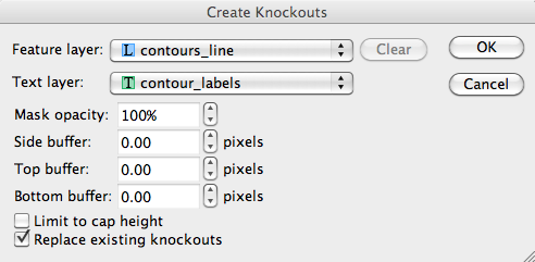
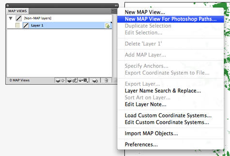
In the MAP Views panel options menu, click “New MAP View For Photoshop Paths…”

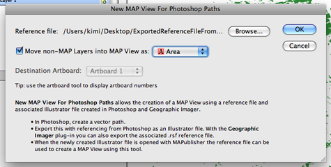
Browse for the exported reference file (either *.tab or *.rsf format from Step 4). Then select “Area” as the feature type for the MAP layer to be created.

The georeference information from the original image is now inherited by the work path objects in the Adobe Illustrator file.

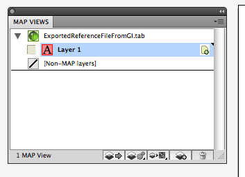
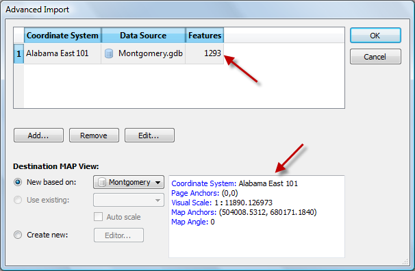
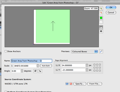
In the MAP View Editor window, you can see all the spatial information such as the coordinate system, scale, and map extent within the artboard. The name for the MAP View is renamed to “Green Area from Photoshop – GI” for Step 8.

At this point, if you have GIS dataset, you can import them to this document. However, I will show you one more MAPublisher trick to bring this green area into an existing MAPublisher file.

7. If you have already made a map with vector dataset, open the Adobe Illustrator file

Keep the Adobe Illustrator file with the work path objects open, then open another Adobe Illustrator file with MAPublisher MAP Objects. Now you have two Adobe Illustrator documents open.

8. Import MAP Objects from the AI file with the workpath to another AI file with a map

Make the Adobe Illustrator document with the map (not with the work path objects) the current document.

On the MAPublisher Toolbar, click the “Import MAP Object” button.

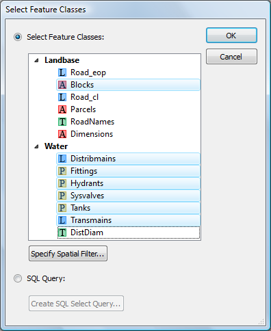
In the “Import MAP Objects” dialog box, select the MAP View “Green Area from Photoshop” and click OK.

All the path objects are imported to the other Adobe Illustrator file with the base map.

However, the imported objects and the base map do not line up appropriately. It is because the scale of the MAP View with the work path and the MAP View with the base map do not match. You can line up those green areas with a simple step.

9. Drag and drop transformation to align the workpath objects geospatially.

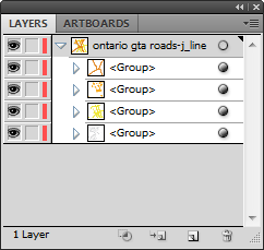
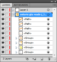
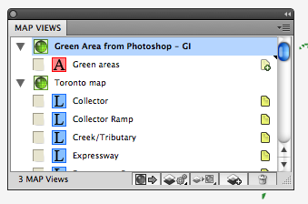
In the MAP Views panel, there are two MAP Views: “Green Area from Photoshop – GI” for the work path imported from another AI file and “Toronto map” for the base map.

Click the MAP Layer “Green areas” in the MAPView “Green Area from Photoshop – GI” …

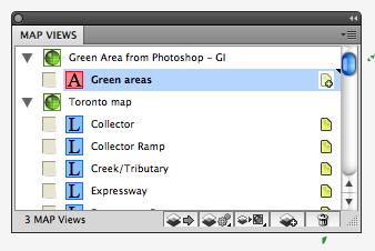
… then drag the map layer to the MAPView “Toronto map”.

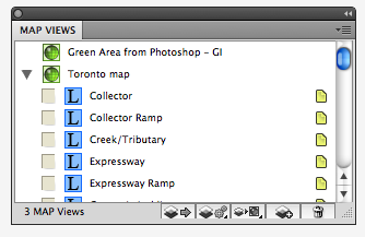
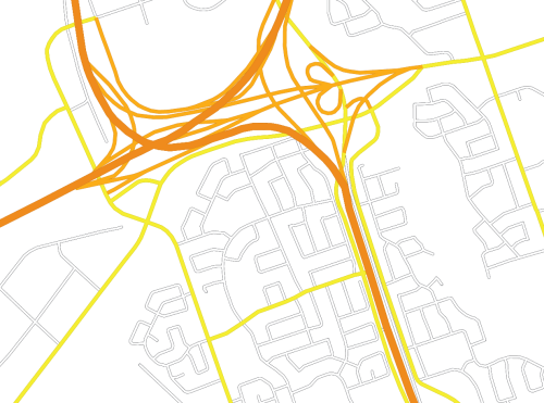
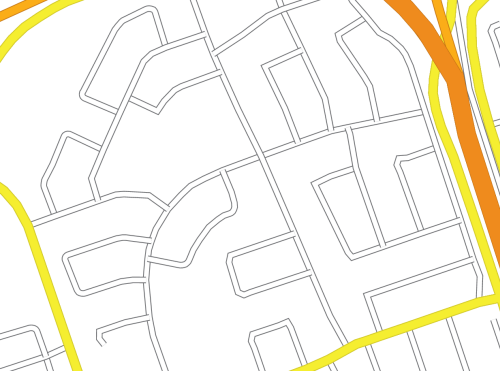
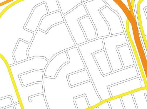
Now all the green areas (work path objects) are lined up nicely with the base map.

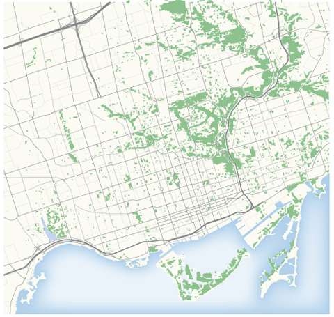
Try this out with your own workflow to see how it may improve your maps.

Creating a false-color composite image with Geographic Imager for Adobe Photoshop

BlogJune 3, 2010

One of the powerful remote sensing tools available in Adobe Photoshop is to detect the land surface information by creating a false color composite image. Multispectral images contain the reflectance information from the visible and invisible electromagnetic spectrum. Using this information, we can detect many kinds of land surface information. For this example, we will detect the green area using Landsat images imported by Geographic Imager for Adobe Photoshop, which ensures all the georeference information is maintained.

Landsat images consist of several gray scale images, with each image containing one of the bands of the electromagnetic spectrum. For example, in the Geographic Imager tutorial folder, there are a set of Landsat images available. Those gray scale images are from Band 1, 2, 3, 4, 5, 7, and 8.

These images need to be combined into one image. The Adobe Photoshop function called “Merge Channels” produces one image by combining mulitple gray scaled images. With this example, those gray scale images from Band 2, 3, and 4 will be merged into one image by assigning a color for each band.

1) Open the Landsat image from Band 2, 3, and 4. Note that the Geographic Imager panel shows the information on the coordinate system and image extents.

2) Open the Channel panel (Window > Channels). Choose “Merge Channels” from the panel options menu.

3) In the Merge Channels dialog box, select RGB color as the mode.

4) In the Merge RGB Channels dialog box, specify the band for each channel: band 4 for the red channel, band 3 for the green channel, and band 2 for the blue channel.

5) As a result, those three images from Band 2, 3, and 4, are assigned to the Blue, Green and Red channels, respectively.

6) Now, let’s take a look at the image!

This combination of false-color makes vegetation appear as red tones. The bright red color indicates the growing vegtation. Water is displayed in a blue color. When the water contains high sediment concentrations, the color will be lighter blue. Urban areas will appear gray to blue-gray in color.

7) All the georeferenced information is inherited by the new image with merged channels from those original images. The georeference information is displayed in the Geographic Imager panel.

Using MAPublisher and Illustrator tools to create great looking road layers

BlogMay 17, 2010

Here’s a question we receive at Avenza support quite often: I’ve located and imported a GIS layer of road lines with attributes for the city I’m mapping. How can I turn this:

into this:

Getting Started

The workflow for this process involves the use of both MAPublisher and Adobe tools, specifically MAP Stylesheets and MAP Selections along with Illustrator’s Graphic Styles and the Appearance Panel.

This process works on roads that have an attribute on which you can base classification rules. My road data has a column named “CLASS” with four categories: Controlled, Controlled-Ramp, Highway, and Street. I’ve created a graphic style for each and loaded them using “Open Graphic Style Library”. I keep the road styles I have created in a template document titled RoadStyles.ai so that I can import the graphic styles I need into whatever map I’m making from my template (see Adobe Graphic Styles Help).

Controlled Access Highway:
Controlled Access Ramp:
Major Road:
Minor Road:

These styles all have been created using the Illustrator Apprearance panel to overlay two strokes, the top stroke with a smaller weight and different colour than the bottom stroke (see Adobe Appearance Panel Help).

With our graphic styles set I can now apply the MAP Stylesheet I built using the following expressions:

Cleaning up with groups

Once we apply these styles using MAPublisher Stylesheets, we will see what steps we muys take to get the appearance we want. Our roads look like this:

but we want them to look like this:

Why does this happen?

This occurs because MAP Stylesheets applies graphic styles at the path level. To look like intersections, each road classification must become one object, whether by being grouped or by turning the various paths into a compound path. Grouping is the preferred method for managing these objects since a compund path will delete the attributes of all paths that are being compounded. In this case, the street names field would be blank for our compound path object as dozens of streets are turned into one compund path. The consequence of this would be to make automatic labelling with MAPublisher Label Pro impossible. A set of paths turned into a group will not have their attributes available to MAPublisher while in a group, however these objects can always be ungrouped making individual paths and their original attributes available again.

Grouping Objects

In order to group our road classes we will have to select the road paths belonging to each class. The expressions we created when defining our MAP Stylesheet rules are available to us to use again through the Expression Library (new in MAPublisher 8.3). We can use MAP Selections to individually select each of our road classes. Once selected the street classes can be grouped using CTRL+G on your keyboard or Object > Group from the menu (See Adobe Group Help). The final step is to re-apply the graphic style appropriate to each group using the Adobe Graphic Style panel.

If we want to get technical here in considering what has happend to our artwork, using the Appearance panel we can see that each of the paths we initially imported now has a graphic style applied to it on two levels: at the path level (done through MAP Stylesheets) and at the group level (done by grouping and applying a graphic style to the group). It is possible to symbolize our artwork even further, at the layer level, by slecting the target symbol for our roads layer (See Adobe Layers Help). If desired we could apply a transparency at the layer level that would supersede all graphic styles used on objects in the layer. Our artwork will now have symbolization that suggests intersections, giving our road map a much neater appearance.

Tweaking

Now that our roads are grouped together, they are much easier to manage in the Illustrator Layers panel.

Groups can be stacked easily. My preference is to arrange with minor roads at the bottom, increasing to multi-laned divided highways at the top of the hierarchy. With our objects grouped it is easy to move objects between groups. Any path can be selected using the Direct Selection Tool and dragged in the Layers panel between groups. This is much simplier than having to use the Appearance panel to strip the path of both graphic styles and apply the desired style. There will be some situations where we will need to override the intersection appearances that result from grouping. In this image we have onramps that definitely do not interesect as this line work suggests!

To do this we must select the road lines that will be on top of the intersection, and using the Illustrator Layers panel, drag them from their group (it does not matter where in the layer hierarchy the are placed).

Our ungrouped ramps can now be sent backwards and forwards relative to other paths, giving a truer representation of the road network:

Using MAP Stylesheets to create a Legend

So why use stylesheets if we must manually group the objects after use? For a few reasons: it keeps us organized, it adds the expressions to the expression library, and most importantly MAP Stylesheets can automatically generate a Legend for us that reflects our Stylesheet rule names:

Good luck creating customized road styles! A deeper understanding of the Illustrator object styling hierarchy can go a long way in helping you use MAPublisher to leverage your GIS datasets!

Create Knockouts with MAPublisher 8.3

BlogMay 3, 2010

We receive many questions about cartographic techniques. A very popular question from MAPublisher users is “How do I mask lines behind contour labels?”

Adobe Illustrator provided some tools to achieve that through a pretty complicated workflow, so we decided to create our own tool! The upcoming release of MAPublisher 8.3 has a very handy new feature called Create Knockouts, here is how it works.

First, you need a labelled map – for example contours and labels.

Start the Create Knockouts tool. All you need to do is choose the layer that contains the lines to be masked and the text layer with the labels.

There are many options available, but let’s keep the default (100% opacity, no buffer around the text, use the default text bounding box from Adobe).

The result:

These knockouts are little bit tight after all, maybe we should add some buffer distance on the side. Start Create Knockouts again (no undo required!). Choose a side buffer of 5 pixels, and make sure to check “Replace existing knockouts”.

Et voilà!

MAPublisher 8.3 is releasing very soon. Watch our Twitter and News page for announcements.

Avenza State Plane Coordinate System Map

BlogApril 19, 2010

MAPublisher and Geographic Imager provide an extensive library of predefined coordinate systems available for referencing or transforming mapping projects.

In the United States, the NGS (National Geodetic Survey), a department of NOAA (National Oceanic and Atmospheric Administration) has established a system that divides the United States into 124 zones, each with its own custom projected coordinate system. This system is known as the State Plane Coordinate System. It is important to note that there are two sets of State Plane coordinate systems defined in the United States, one based on the North American Datum of 1927 and the other based on the North American Datum of 1983. In addition to NAD 83, the NAD83 HARN and NSRS2007 adjustments are available for use. All three versions of NAD83 are available in metres, feet or international feet.

State Plane Coorindate Systems projections

There are four projections for SPCS. The geometric direction of each state determines the projection utilized. For states that are longer in the east-west direction, the Lambert Conformal Conic is used. States which are longer in the north-south direction use the Transverse Mercator projection. The panhandle of Alaska, which has the sole distinction of lying at an angle, garners the use of the Oblique Mercator projection, while Guam uses a Polyconic projection.

These coordinates systems are all defined in the MAPublisher and Geographic Imager library, however the initial question “which one do I need to use for my map” cannot be answered by the software itself.

There are a number of ways to determine in which zone your American area of interest lies. One online resource, searchable by latitude and longitude coordinates, can be found on this NGS website.

In an effort to better assist mapmakers in their selection of the appropriate system, the Avenza support team has prepared a searchable interactive map using MAPublisher 8.2 MAP Web Author tool. View the SPCS map here.

A MAPublisher geospatial PDF of the same map is also available for download here.

Transform into State Plane Coorindate Systems using MAPublisher

When it comes time to transform your data into the appropriate State Plane Coordinate System zone, use the MAP View Editor Perform Coordinates System Transformation option. When you specify the destination coordinate system for the transformation, navigate to Coordinate Systems > Projected > North America > United States > US State Plane NAD 83 – on the right hand list, you’ll find all the state plane zones sorted by state name and zone name: select the right one!

Note: similarly you can select the NAD27 state plane systems from Coordinate Systems > Projected > North America > United States > US State Plane NAD 27 if appropriate.

Improved Reprojection Engine in MAPublisher 8.3

BlogApril 9, 2010

One of the exciting new changes in MAPublisher 8.3 is that we’ve substantially rewritten our reprojection engine. What I’d like to do here is explain what the changes are, and what they mean for you, the user.

The old reprojection engine was point-by-point. Essentially, we walked each path and simply reprojected each point one by one. This simple approach works very well but it has one important deficiency: it lacks context. The internal reprojection system never sees anything more than a single point, and therefore is limited to just reprojecting.

So what is the new system doing? Our new reprojection engine is performed feature-by-feature. This is important because it means the internal system no longer just sees a single point, but rather a collection of points and how they are arranged. This means it can notice things like an area that wraps around to the other side of the world! In the old system, it would just blindly punch out points, and if a path suddenly jumped to the other side of the page, well, that’s where the path went. But now the reprojection engine can notice things like that, and clip the art appropriately. If necessary, it will even break a single path into a compound path! But it’s probably easier to understand if we demonstrate it visually.

Here is a map of Canada with two layers: rivers & provinces. Both sets of art are coloured nicely and the provinces layer even has an opacity reduction to make the rivers stand out a little.

I’ve created a new coordinate system I’ve called ‘Miller Cylindrical Shifted’. I just made a copy of the ‘Miller Cylindrical’ coordinate system and then altered my copy’s central meridian to be 90 instead of zero. I did this so that if I reproject Canada into ‘Miller Cylindrical Shifted’, half of Canada should be on the left-hand side, and half should be on the right-hand side. Let’s see how MAPublisher 8.2 handles it:

Yikes! The old reprojection engine had no idea that some of those lines were going off the end of the projection’s envelope!

Now let’s try it in MAPublisher 8.3 with the new reprojection engine:

Wow! What a difference feature-by-feature makes! The new engine recognizes that those paths needed to be clipped and properly split polygons and lines as needed. It’s also important to note that the areas & lines are still intact. e.g. Northwest Territories was split, but it’s still a single compound path with all of its islands — some of those islands have simply been split into pieces. The split even preserves all the original path’s properties, including attributes and styles!

Import Geodatabase Feature Classes into Adobe Illustrator

BlogMarch 9, 2010

In this post, we’ll cover how simple it is to import a geodatabase feature class into Adobe Illustrator using MAPublisher import tools enabled with the Spatial Database add-on.

Spatial databases are optimized data repositories for spatial data storage and management. Many GIS environments use spatial databases to easily access and manage GIS data in a central location.

MAPublisher 8.2 introduces support for import of the popular ESRI single-user and multi-user Geodatabases: Personal, File and ArcSDE Geodatabases; and direct access to ArcSDE server. The MAPublisher Spatial Database importer is built on ESRI software libraries and requires a valid ESRI software and license installed on the computer (ArcGIS 9.2 and higher).

To import one, you can use either Simple Import or Advanced Import. In this scenario, we’ll use Advanced Import. When we add data, a list of Geodatabase types are located at the bottom of the Format list. We’ll be importing some feature classes from a simple geodatabase consisting of waterlines, hydrants and valves.

After browsing for the geodatabase (a File geodatabase in this case), the Select Feature Classes dialog box appears. We’ll go ahead and select a few feature classes from the Landbase and Water feature sets listed.

The Advanced Import dialog box shows the number of features being imported and the coordinate system as well as page and map anchors.

The features are imported and are ready to be used in a map.

Avenza maps makes it easy to interact with offline
maps on your iOS, Android and Windows devices.

Get the app. Get the map.